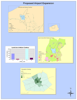
Above: Exercises 1-5 on ArcGIS Tutorial
Had it not been for the very detailed step by step instructions on on the tutorial for the ArcGIS Software, I am certain I would have been lost. I have always considered myself to be a computer savvy person, but after this tutorial I realize I still have MUCH to learn. Organization is probably the most important element in this process, as a lack of organization can have its consequences. I ran into one little set back strictly because I was not as organized as I should have been with my folders from the very beginning. This being something completely new for me, I realize the only way to really become comfortable with the software is through a process of trial and error. Making mistakes, and leaning how to fix them has always been the best way for me to learn. I have so far only gone though the tutorial one time, and I plan on spending a lot more time the next few times I go through it and playing around with the different features a but more.
It took me a couple of hours just to figure out how to use the remote access and work on the UCLA network from home. Just the fact that I was able to remotely access the computers in the UCLA labs from so far away amazed me. The fact that you can only access the computers after hours really put some time constraints on me, which was somewhat frustrating because I couldn't get things done when I had time to do them during the day. I guess the luxury of having such an advanced technology at your fingertips has to have certain drawbacks, and for me this was one.
Prior to this tutorial, I knew absolutely nothing about ArcGIS and did not realize how very helpful in solving real-life problems programs like this one are. It was really interesting to see the process first hand, and to have a hands on introduction to the software. It was very quick and easy when being guided through the steps, especially because the information we were working with was so easily at our disposal. There will not be many instances, I am sure, where the data to take on a project such as noise levels in airport expansion will be so readily available. The real test will come when I have to start from scratch.
Overall, it was exciting to have this introduction into using the Arc GIS software. Obviously I feel more comfortable using the software after the tutorial than before because I had no prior knowledge about it. It is without a doubt complex, and I will need to continue referring back to what I learned in these 5 exercises for future reference.


 The above map represents the black population in U.S. counties with the darker shades of green representing more concentrated areas. The southeastern United States clearly shows the highest concentrations in Black population for the 200o Census, with data collected in 1999. The states of Louisiana, Georgia, Mississippi, Alabama, South Carolina, and North Carolina seem to have the most counties with 46.68% - 86.49% of the total population self-reported as Black. Many counties in Texas, Florida, and Tennessee had a self-reported Black population of 24.57% - 46.33%, with the rest of the U.S. having significantly lower populations. There are only 4 tiers of color, which is enough to give an overall idea of where the concentrations are. Another tier of color would give a bit more specificity and allow us to further see the trends in population densities.
 Data for the above map of self-reported Asian population in the U.S. was also taken for the 2000 Census. It shows the highest concentrations in dark purple, and lower concentrations with lighter shades. California and Hawaii have the most counties with an Asian population of 17.57% - 46.04%, with other states on the west coast following closely behind. This data could be more telling if there was another level of color. The darkest states could have 17.57% Asian population, but could just as well be 46.04% Asian. It is a large difference in population to be covered by a single tier. An added level would be able to illustrate the percentages better. The New York/New Jersey area also had higher Asian concentrations than that surrounding counties. There are lower concentrations of Asians, in comparison to Blacks because in the 2000 census they had a lower total population.
  This last map illustrates "some other race" population by percentage for the 2000 Census. Given that the Census does not offer a "Hispanic" or "Latino" option to self-report, and given the areas that show the most dense populations of "some other race," one can infer that the data is reporting the majority of the Hispanic population of the U.S. Anyone who does not identify with any of the other options to choose from can self-report as "some other race," so it also includes people that identify themselves as something other than Hispanic. The highest concentrations occurred in the states of California, Arizona, New Mexico, and Texas - with the most counties in the 10.08% - 20.87% and 20.88% - 30.08% tiers. These are all states that share a boundary with Mexico, which gives some more indication of who "some other race" may be. There are also denser concentrations in the northwest (western U.S. in general), Florida, and the New York area.
 Above: Equal-Area World Map Projections illustrating distance from Washington D.C. to Kabul.

 These are elevation estimates for the 3771000 UTM northing, with the two elevations at the easting intersections that pass through UCLA labeled.
 14. What is the magnetic declination of the map?